

Three countries, three dialects of meaning, one curious tourist.
Prologue — Why a Tourist?
Every traveler carries a notebook. Mine is filled with scatterplots, token lists, and vector embeddings — souvenirs from three very different countries I have been wandering through lately. Each one promises to make sense of the world in its own dialect: one through numbers, one through words, and one through the strange new mathematics of meaning itself.
I won’t pretend to have mastered the language of any of them — a tourist rarely does — but I have come back with enough to sketch the shape of the landscape, the customs of the locals, and the few souvenirs worth carrying home. Pack light. Bring your curiosity. We begin in a country built entirely of numbers.
Stop 1 — The Country of Numbers
“In the country of numbers, every house has a number on its door and every door tells you something true. The trouble is knowing which doors to knock on.”
Our first dataset is twenty-five years of country-level indicators — energy, climate, GDP, population, twenty-two columns in all. Like any tourist arriving in a new city, the temptation is to photograph everything. But not every monument is worth the film. Our question is small but stubborn: what makes a country’s CO₂ emissions go up?
The Scatterplot — A Tourist’s First Window
In 1854, London physician John Snow mapped cholera deaths during an outbreak in Soho. The deaths were concentrated around a specific public water pump, providing evidence that cholera spread through contaminated water rather than through air. The modern scatterplot follows the same basic principle: plotting observations spatially or numerically to identify relationships, clusters, and correlations between variables.
I plotted GDP against CO₂ emissions and the result was lopsided. Some economies are much larger than others they dominate the plot so much that a clear pattern cannot be seen.
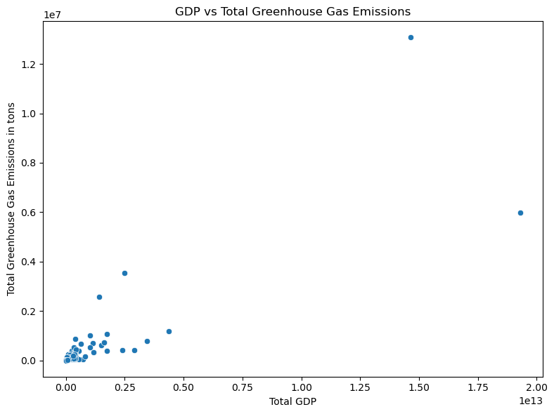
The Trick of the Logarithm
This is the kind of data logarithms are for. The increase in the dependent variable doesn’t happen directly proportional to the increase in the independent variable. In a sense once converted to log scale we are seeing relative change instead of absolute change.
Plotting both axes on log scale rearranges the world: instead of asking “how much CO₂ does this country emit?”, the chart now asks “how does emission grow as the economy grows, in proportional terms?”
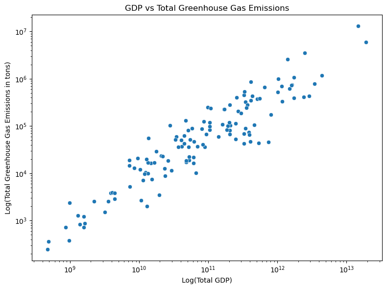
A Linear Relationship shows up. A constant percentage increase in GDP corresponds to a constant percentage increase in CO₂. So for an increase in GDP by 80% might Increase the CO2 by 50%. The correct relation we will find later when we reach Regression model.
The Correlation Heatmap — A Social Diagram of the Data
Before we model anything, it is worth asking which variables in this country are on speaking terms.
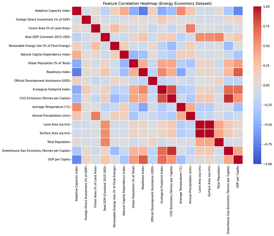
Correlation measures how predictably one variable moves with another. A correlation of +1 means perfect lockstep; −1 means perfect opposition; 0 means they ignore each other. Two cautions every tourist should be told at the city gate:
Correlation captures only linear friendships. Two variables can be deeply, intricately related and still show a correlation near zero — if their friendship is curved. The relationship between caffeine intake and alertness, for example, peaks and then collapses. The correlation coefficient will be politely confused.
Correlation is not causation. This is the warning every introductory statistics course tries to emphasize, yet it is frequently ignored in public debate and media reporting. A famous example of a spurious correlation is that between 1999 and 2009, the number of films Nicolas Cage appeared in closely tracked the number of people who drowned in swimming pools each year. Neither caused the other; the variables simply happened to move in similar ways over the same period.
A different kind of example involves ice cream sales and shark attacks. Both tend to increase during the summer months, but ice cream consumption does not cause shark attacks. Instead, both are influenced by a third variable: hot weather increases beach attendance, which in turn raises both ice cream purchases and the number of people swimming in the ocean.
The distinction matters. Sometimes two variables are unrelated and merely coincide statistically; other times they are connected indirectly through a hidden or confounding variable. In either case, correlation is a starting point for investigation, not proof of causation.
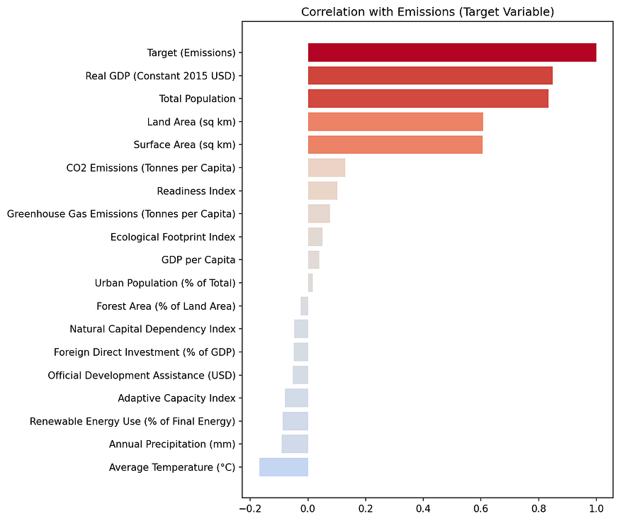
For our purposes: which variables are most correlated with total CO₂ emissions? Three stand out. Surface area and land area turn out to be the same variable wearing different clothes, so we keep one. GDP, population, and land area survive as candidates for the regression.
Linear Regression — Drawing the Straightest Road
Linear regression is the most modest of models. It assumes the relationship between input and output is a straight line, and finds the line that hurts least. It is high bias, low variance. High bias meaning it assumes the relationship is linear hence would not find other types of non linear relationships even if it exists. Low variance means the values don’t change wildly with new data.
Before training, we split the data 80/20.
Train and test, or why you don’t grade yourself. Imagine you are studying for an exam using last year’s paper. You memorize every question. On exam day, the paper is different. If you can still answer well, you’ve learned the subject. If you can only repeat last year’s answers, you have memorized — and memorization is what we call overfitting in machine learning. The test set exists to be a fresh paper the model has never seen.
from sklearn.linear_model import LinearRegression
from sklearn.model_selection import train_test_split

X = df_model[["log_gdp"]]
y = df_model["log_emissions"]
X_train, X_test, y_train, y_test = train_test_split(
    X, y, test_size=0.2, random_state=42
)
model = LinearRegression()
model.fit(X_train, y_train)
(random_state=42 is a small joke between data scientists — Douglas Adams’s Hitchhiker’s Guide picked 42 as “the answer to life, the universe, and everything.” Any integer works; this one comes with the warm feeling of being in on the reference.)
Judging the Model — Three Rulers, Three Stories
A trained model needs a verdict. Three measurements help us reach one.
R² — the “how much better than guessing?” score. Imagine a friend who always guesses the average temperature for tomorrow as 22 °C, every day, year-round. Their forecast is mediocre but not random — it beats guessing 5 °C in summer. R² asks how much your model improves on that lazy friend. An R² of 0 means you’ve matched the lazy friend exactly. An R² of 1 means perfection. An R² of 0.9 means you have explained 90% of the day-to-day variation they could not.
R² = 1 − (Σ (yᵢ − ŷᵢ)²) / (Σ (yᵢ − ȳ)²)
The above Formula is used to calculate R2 score.
yᵢ = Actual Values
ŷᵢ = Predicted Values By the Model
ȳ = Mean of values in the Y axis
MAE — Mean Absolute Error. The average size of your mistakes, in the same units as the thing you are predicting. If your house-price model has an MAE of ₹3 lakhs, your typical mistake is ₹3 lakhs in either direction. MAE is forgiving toward outliers — a single ₹50-lakh miss is just one item in the average.
MAE = (1/n) Σ |yᵢ − ŷᵢ|
RMSE — Root Mean Squared Error. The same idea, but it squares the errors first. A ₹50-lakh miss now counts not 50 times worse but 2,500 times worse than a ₹1-lakh miss. RMSE is the metric for situations where one catastrophic failure is worse than many small ones. (Air traffic control prefers RMSE. So does anyone forecasting hurricanes.)
RMSE = √[(1/n) Σ (yᵢ − ŷᵢ)²]
I trained four versions of the model, each with a different combination of features, to see what each ingredient actually contributes:
| Model  | Train R²| Test R²| Train MAE| Test MAE| Train RMSE | Test RMSE |
| -------| --------| -------| ---------| --------| ---------- | --------- |
| Model 1| 0.886   | 0.749  | 0.601    | 0.714   | 0.739      | 0.873     |
| Model 2| 0.935   | 0.890  | 0.447    | 0.436   | 0.557      | 0.579     |
| Model 3| 0.942   | 0.891  | 0.408    | 0.427   | 0.529      | 0.574     |
| Model 4| 0.883   | 0.840  | 0.603    | 0.526   | 0.748      | 0.696     |
Since the model was trained on the logarithm of CO₂ emissions, the reported MAE and RMSE are in log units rather than tons of CO₂
The postcard worth sending home: GDP alone is a mediocre fortune-teller (R² 0.75), but GDP and population together climb to 0.89. Adding land area on top of that buys almost nothing. Population is doing real explanatory work that GDP alone misses — which makes intuitive sense, since two countries with identical GDP but vastly different populations are likely to live, drive, and burn fuel quite differently.
The gap between training and test scores is modest, which means the model has resisted the temptation to memorize. A respectable baseline, then. Not the last word, but a solid first one.
Stop 2 — The Library of Legal Texts
“If the country of numbers had street signs at every corner, the library of legal texts has none. The names of things are not given to you; you have to listen for them.”
The second stop takes us somewhere stranger. The dataset is no longer rows and columns — it is a stack of Supreme Court judgments from Indian Kanoon, each one a long formal document written in the particular dialect of Indian legal English. No labels. No obvious structure. Just text.
The tourist’s question changes accordingly. We no longer ask “can we predict this number?” We ask “what is this collection actually about?”
Extraction — Opening the Books
Every PDF must first be coaxed into plain text. PyMuPDF handles the extraction; the results — filename, year, raw text — go into a pandas Dataframe. The Dataframe is then pickled, because re-extracting hundreds of PDFs every time the session restarts is a kind of low-grade suffering nobody should endure twice.
Cleaning — Clearing the Underbrush
A short story about stop words. In 1958, an IBM researcher named Hans Peter Luhn was building one of the first automatic indexing systems and noticed that the most frequent words in English — the, of, and, a, to — appeared so often they carried almost no information. They were like background noise at a café: present in every conversation, distinctive of none. He called them stop words and proposed throwing them away. The idea stuck, and many traditional NLP pipelines start this way.
Legal text has its own background noise on top of the standard one: court, judgment, petitioner, respondent, learned counsel. These appear in nearly every document, so they fail to distinguish one case from another. We add them to the standard list.
legal_stopwords = {
    "court","judge","justice","section","petitioner","respondent",
    "case","law","india","http","org","kanoon",
    "hereby","thereof","therein","wherein","said",
    "learned","counsel","appeal","judgment","honble",
    "supreme","high","would","also","may","shall"
}
Then we tokenize (split text into individual words), lemmatize (collapse running, ran, runs into a single root, run, the way a librarian files three editions of a book under one title), and use bigrams — pairs of words that travel together so often they are effectively one concept. Sale_deed is not a sale followed by a deed; it is a single legal instrument. New_York is not a fresh York. Arbitration_agreement, corporate_debtor, financial_creditor — the bigram model spots these and treats them as the units they actually are.
Topic Modelling with LDA — Listening for Patterns
Imagine you walk into a vast cocktail party where dozens of conversations are happening at once. You cannot follow any single one, but if you stand still and listen, certain word-clusters drift past you: quarterly, revenue, board from one corner; bail, accused, custody from another; plaintiff, possession, Sale_deed from a third. Without ever joining a conversation, you can guess what each group is talking about.
Latent Dirichlet Allocation (LDA) is the algorithm that does this listening for us. Its assumption is elegant: every document is a mixture of topics, and every topic is a mixture of words. You tell it how many topics to find, and it reverse-engineers both distributions from the data alone.
from gensim.models import LdaModel

lda_model = LdaModel(
    corpus=corpus,
    id2word=dictionary,
    num_topics=10,
    passes=10,
    random_state=42
)
The output is a list of word distributions — one per topic. LDA refuses to name the topics for you; that part is your job. You look at the words, recognize the family, and supply a label.
Here is what I heard the library whispering back:
Topic 0: 0.012*"assessee" + 0.010*"tax" + 0.010*"bank" + 0.007*"income_tax" + 0.006*"income" + 0.005*"business" + 0.005*"revenue" + 0.004*"agreement" + 0.004*"sale" + 0.004*"company"
Topic 1: 0.009*"employee" + 0.008*"post" + 0.007*"appointment" + 0.005*"candidate" + 0.005*"tribunal" + 0.004*"contract" + 0.004*"commission" + 0.003*"appointed" + 0.003*"division_bench" + 0.003*"category"
Topic 2: 0.024*"company" + 0.007*"offence" + 0.006*"election" + 0.006*"board" + 0.006*"complaint" + 0.005*"director" + 0.005*"detention" + 0.004*"regulation" + 0.004*"member" + 0.003*"accused"
Topic 3: 0.017*"arbitration" + 0.012*"award" + 0.008*"child" + 0.008*"agreement" + 0.008*"contract" + 0.008*"arbitrator" + 0.006*"arbitral_tribunal" + 0.005*"arbitration_agreement" + 0.004*"tribunal" + 0.003*"claimant"
Topic 4: 0.009*"constitution" + 0.008*"regulation" + 0.007*"institution" + 0.007*"university" + 0.006*"member" + 0.005*"education" + 0.004*"committee" + 0.004*"legislature" + 0.004*"candidate" + 0.004*"commission"
Topic 5: 0.009*"candidate" + 0.005*"investigation" + 0.005*"ngt" + 0.004*"project" + 0.004*"examination" + 0.003*"board" + 0.003*"mark" + 0.003*"police" + 0.003*"tribunal" + 0.003*"committee"
Topic 6: 0.016*"suit" + 0.015*"plaintiff" + 0.015*"land" + 0.013*"defendant" + 0.008*"possession" + 0.004*"decree" + 0.004*"agreement" + 0.004*"sale_deed" + 0.003*"sale" + 0.003*"tenant"
Topic 7: 0.028*"accused" + 0.016*"bail" + 0.007*"deceased" + 0.007*"offence" + 0.004*"grant_bail" + 0.004*"compensation" + 0.004*"sentence" + 0.004*"custody" + 0.004*"magistrate" + 0.004*"victim"
Topic 8: 0.011*"corporate_debtor" + 0.007*"company" + 0.007*"resolution_plan" + 0.006*"ibc" + 0.005*"bank" + 0.005*"good" + 0.005*"adjudicating_authority" + 0.005*"creditor" + 0.004*"financial_creditor" + 0.004*"tax"
Topic 9: 0.027*"accused" + 0.008*"offence" + 0.008*"witness" + 0.008*"police" + 0.008*"prosecution" + 0.007*"deceased" + 0.007*"investigation" + 0.005*"ipc" + 0.005*"complaint" + 0.005*"fir"
This is the moment the library reveals itself. With no supervision, no labels, no training on legal taxonomy, LDA has carved the Supreme Court’s caseload into ten recognizable domains of Indian jurisprudence. A practicing lawyer reading this list would nod. That, I think, is the postcard worth sending home from this stop.
A Brief History — Where LDA Came From
The paper that introduced LDA is one of the most cited in machine learning history. David Blei, Andrew Ng, and Michael Jordan published “Latent Dirichlet Allocation” in the Journal of Machine Learning Research in January 2003, and it has since been cited over sixty thousand times. (Andrew Ng would later co-found Coursera and become one of the most recognizable voices in AI education; Michael Jordan is the Berkeley professor whose students populate much of modern machine learning’s leadership.)
The original paper, for the curious: Blei, D. M., Ng, A. Y., & Jordan, M. I. (2003). Latent Dirichlet Allocation. Journal of Machine Learning Research, 3, 993–1022. https://www.jmlr.org/papers/volume3/blei03a/blei03a.pdf
LDA generates topics by relying on the idea that words which frequently appear in the same documents are likely associated with a common underlying theme. It then infers hidden topics that best explain these word co-occurrence patterns across the corpus, and represents each topic as a distribution over words
LDA assumes a document is a collection of topics and a topic is collection of words. Technically speaking a document is multinomial distribution on topics and a topic is a multinomial distribution of words.
LDA process tries to learn the word distribution and topic distribution. The “Dirichlet” in LDA refers to the Dirichlet distribution. It is a probability distribution over probability distributions. In LDA, it is used as a prior to generate:
- the topic mixture for each document
- the word distribution for each topic
For example, if we assume three topics, a document’s topic mixture might look like [0.7, 0.2, 0.1], where each value represents the proportion of topic 1, topic 2, and topic 3 in that document. There is an assumption that topic mixtures are usually sparse, meaning a document is likely dominated by one or a few topics rather than having all topics equally represented.
During training, LDA does not directly assign topics based on word adjacency. Instead, it iteratively infers:
- which topic each word in a document is likely associated with
- based on how frequently that word appears in different topics across the entire corpus, and how dominant those topics are within the document
From this iterative process, LDA learns:
- the topic distribution for each document
- the word distribution for each topic
These are the learned latent structures that explain how words are distributed across documents
LDA and the Large Language Models — Same Question, Different Answers
It is fair to ask: in an age when you can paste a thousand legal judgments into a large language model and simply ask “what are the main themes?”, why bother with a twenty-year-old probabilistic model?
The honest answer is that LDA and LLMs are answering the same question with radically different tools, and the differences matter.
LDA is a bag of words. It does not know that contract and agreement mean similar things. It does not know what order words appeared in. It cannot read context. It is, in a sense, a very sophisticated word-counter — it watches which words tend to cluster together across thousands of documents and reverse-engineers the clusters.
LLMs are readers. They were trained on more text than any human will read in a lifetime, and somewhere in that training they absorbed not just word patterns but grammar, world knowledge, and a kind of statistical mimicry of reasoning. Ask GPT-4 or Claude to find themes in a corpus and it will read each document, understand it the way a fluent intern would, and write you a summary.
So when do you reach for which? Below are some of the factors that decide
Interpretability — can I see why it chose a topic?
LDA: Yes, every topic is a word distribution you can inspect
LLM: Mostly no, it’s a black box
Cost & speed
LDA: Cheap, runs on a CPU, scales to millions of documents in minutes
LLM: Expensive, GPU-bound, slow at scale
Stability — same input, same output?
LDA: Yes, deterministic given a seed
LLM: Drifts between runs, even at temperature 0
Semantic understanding — synonyms, paraphrases?
LDA: No
LLM: Yes
Unsupervised at scale — 100k documents, find structure?
LDA: Excellent
LLM: Possible but expensive
Generating fluent text
LDA: Cannot
LLM: Excellent
Where LDA Still Earns Its Keep
LDA’s death has been quietly exaggerated. It is still the right tool in several places:
- Exploring an unknown corpus quickly. You inherit ten thousand customer support tickets, or a decade of internal memos, or a folder of regulatory filings. Before you can ask intelligent questions, you need a map. LDA produces that map in minutes, on a laptop, for free.
- Tracking topics over time. Dynamic topic models are still the cleanest way to ask “how did the conversation in this corpus shift between 2010 and 2025?” — useful for news analysis, scientific literature reviews, social media trend monitoring, and regulatory drift studies.
- High-volume routing where interpretability matters. Insurance claim categorization, legal document triage, helpdesk ticket assignment. If a regulator asks “why was this case flagged?”, the answer “because words like assesses, income tax, revenue dominated” is defensible. “Because the LLM said so” is not.
- Preprocessing for LLM pipelines. A common modern pattern is to use LDA to bucket millions of documents into a dozen broad topics first, then route each bucket to a specialized LLM workflow. LDA is the cheap front door; the LLM is the expensive specialist behind it.
- Anywhere you need to defend the result to a non-technical audience. A printable topic-and-keywords list is something a lawyer, doctor, or compliance officer can read and verify. A neural network’s hidden state is not.
The lesson, perhaps, is that machine learning rarely replaces its old tools entirely. It accumulates them. The tourist who knows only the newest dialect will miss what the older one still says best.
Stop 3 — The Vector Realm
“At the third stop, words stop being words. They become coordinates. You no longer ask what a sentence says — you ask where it lives.”
The final leg is the strangest. Classical NLP — the kind we just did with LDA — counts words. It knows that contract and agreement are different tokens, even though every lawyer knows they often mean the same thing. To bridge that gap, we leave the country of words entirely and enter the country of vectors.
Embeddings — Words as Coordinates
A small miracle from 2013. A team at Google trained a model called word2vec on a few billion words of news text and discovered something nobody had quite predicted. They could do arithmetic with words. If you took the vector for king, subtracted man, and added woman, the resulting vector pointed almost exactly to queen. Paris − France + Italy = Rome. Walking − walked + swam = swimming. The model had never been told what gender or geography were. It had only read a lot of sentences, and in trying to predict which words appeared near which, it had assembled a geometry of meaning by accident.
An embedding model is a neural network trained to convert any piece of text — a word, a sentence, a paragraph — into a long list of numbers (a vector, usually 384 to 1,536 dimensions). What makes the space useful is how the vectors are arranged. Sentences with similar meaning end up close together, regardless of whether they share vocabulary at all.
So “the buyer paid for the property” lives near “consideration was tendered for the immovable asset” — even though they share almost no words. The geometry has done what counting could not.
Cosine Similarity — Measuring Closeness in a Thousand Dimensions
How do you measure “closeness” between two vectors in a space with hundreds of dimensions? You cannot visualize it, but the math is surprisingly simple. Picture two arrows leaving a single point. The closer the directions they point, the more similar they are. The cosine of the angle between them is +1 when they point the same way, 0 when they are perpendicular (unrelated), and −1 when they point exactly opposite ways.
Cosine Similarity = A.B / |A||B|
Division by length means we care only about direction, not magnitude. A short arrow and a long arrow pointing the same way are treated as equally aligned — which is what we want, because the length of a sentence’s embedding should not matter; only its meaning should. For semantic search, anything above ~0.7 often suggest the two pieces of text have good similarity in what they are talking about.
Chunking — Cutting Long Scrolls into Pages
Supreme Court judgments are long — often dozens of pages. Embedding an entire document into a single vector loses too much detail, because the embedding becomes an average of everything inside. The signal washes out. (Imagine summarizing a novel as a single sentence — accurate, perhaps, but useless for finding any specific scene.)
So we slice each judgment into overlapping 500-word chunks, with a 100-word overlap so an idea sitting on a chunk boundary is not cut in half:
def chunk_text(text, chunk_size=500, overlap=100):
    words = text.split()
    chunks = []
    step = chunk_size - overlap
    for i in range(0, len(words), step):
        chunks.append(" ".join(words[i:i + chunk_size]))
    return chunks
Each chunk keeps a reference back to its parent document, so we can answer not just “what does this passage say?” but “which judgment is this from?”
Indexing with FAISS — Building the City’s Address Book
Once every chunk is embedded, we have a forest of vectors — possibly hundreds of thousands of them — and we need to find the nearest neighbours of any given query, fast. Comparing a query against every vector one by one works for a few thousand, but at scale you need something smarter.
FAISS (Facebook AI Similarity Search) is the library built for exactly this. Facebook open-sourced it in 2017 after using it internally to search through billions of image and text vectors for tasks like reverse image search and content recommendation. It is the address book that makes the city navigable.
import faiss
import numpy as np

embeddings = np.array(embeddings).astype("float32")
faiss.normalize_L2(embeddings)
dim = embeddings.shape[1]
index = faiss.IndexFlatIP(dim)
index.add(embeddings)
IndexFlatIP is the simplest flavor — an exhaustive inner-product search. For collections in the millions, you would reach for approximate variants (IVF, HNSW), which trade a tiny bit of recall for enormous speed gains. At our scale, exact search is fast enough.
Similarity Search
The final move: a question goes in, the most similar chunks come back, each tagged with the judgment it came from.
def search(query, top_k=10):
    query_vec = model.encode([query]).astype("float32")
    faiss.normalize_L2(query_vec)
    scores, indices = index.search(query_vec, top_k)
    return [
        {
            "file": chunked_data[idx]["file"],
            "year": chunked_data[idx]["year"],
            "chunk": chunked_data[idx]["chunk_text"],
            "score": float(score)
        }
        for score, idx in zip(scores[0], indices[0])
    ]
Ask “Cases Dealing with Freedom of speech under constitution” and the system returns the passages and documents closest to that meaning — not the ones containing those exact words. The library has become searchable in a way that did not exist a decade ago.
The Tourist’s Conclusion
Three countries, three different theories of what understanding the data even means.
- In the country of numbers, understanding is prediction — given GDP and population, guess the emissions.
- In the library of legal texts, understanding is summary — here are the ten conversations this corpus keeps having.
- In the vector realm, understanding is proximity — show me what this question sounds like.
None of them is the whole picture. Each is a dialect, and the modern data analyst is — like any decent tourist — someone who has learned to say hello and where is the train station in all three.
I’ll be back with more postcards.